NOTE: This is a working document that is regularly being edited and added to.

As noted in our discussion of the quadrupole mass filter, in the late 1950's and early 1960's, Wolfgang Paul and collaborators were developing novel methodolgies for storing and manipulating ions through the use of alternating radio frequency electric fields.  Their methodologies utilized quadrupolar fields, which by definition have potentials that scale with the square of x,y and z in a cartesian coordinate system:

$$\begin{equation}\phi(x,y,z) = A(λx^2 + σy^2 + γz^2) + C\end{equation}$$

Because of the Laplace equation/condition, the gradient of the potential must equal zero (at least in the absence of any charges):

$$\begin{equation}\nabla\phi(x,y,z) = 2A(λx + σy + γz) = 0\end{equation}$$

$$\begin{equation}λx + σy + γz = 0\end{equation}$$

This equation can be satisfied in an infinite number of ways, with various values of the coefficients λ, σ and γ.  One of the most well-known solutions utilizes the combination  λ=1, σ=1 and γ=-2 to give a potential of:

$$\begin{equation}\phi(x,y,z) = A\left(x^2 + y^2 - 2z^2\right) + C\end{equation}$$

If this potential is instead expressed in polar coordinates, it takes the form:

$$\begin{equation}\phi(r,z) = A\left(r^2 - 2z^2\right) + C\end{equation}$$

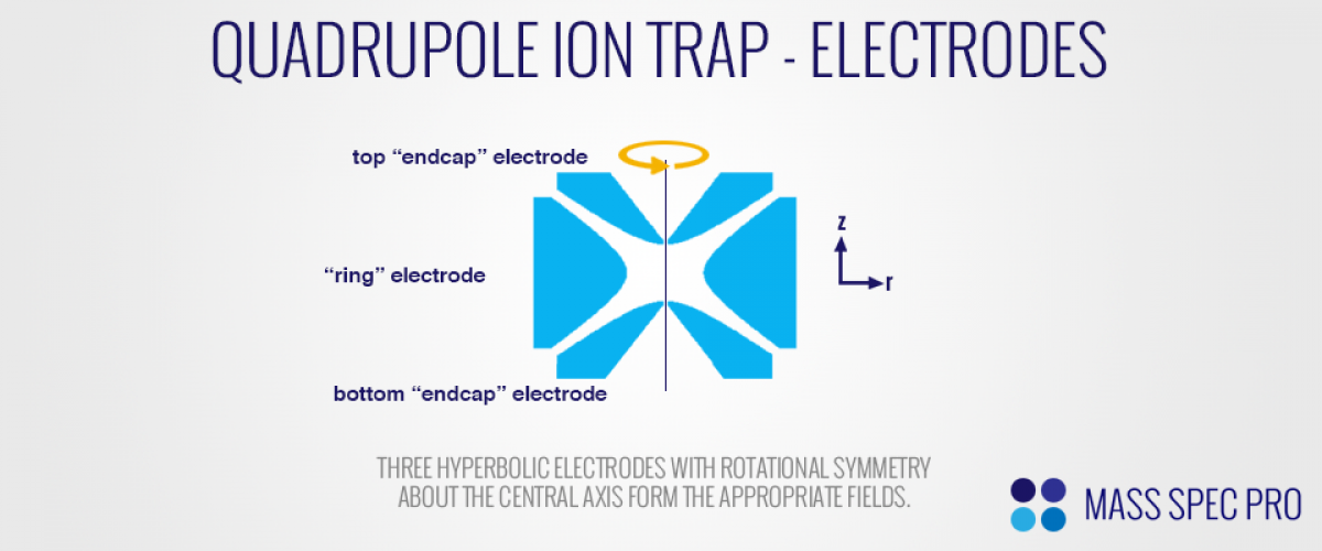
This potential is generated via three rotationally symmetric electrodes with hyperbolic inner surfaces. The center electrode has a donut like shape, and is most often referred to as the "ring" electrode.  It has the general form:

$$\begin{equation}\frac{r^2}{r_0^2} - \frac{2z^2}{r_0^2} = 1\end{equation}$$

The remaining two electrodes reside above and below the ring electrode, and are referred to as the "endcap" electrodes.  They have the general form:

$$\begin{equation}\frac{r^2}{2z_0^2} - \frac{z^2}{z_0^2} = -1\end{equation}$$

Now, we can think more about the exact characteristics of the electric potentials inside the QIT.  We begin by defining the potential $\phi_0$ as the difference between the potentials applied to the ring and endcaps.  For now we will think of the endcaps as both having the same potential applied to them.

$$\begin{equation}\phi_0 = \phi_{ring} - \phi_{endcaps}\end{equation}$$

Now consider the point on the inside face of the ring electrode at $z=0$ and $r=r_0$.  Since this point is on the ring electrode, it will obviously have the potential $\phi_{ring}$.  These facts, combined with the general form of the quadrupole potential (expressed in radial coordinates) provides:

$$\begin{equation}\phi_{ring} = A\left(r_0^2\right) + C\end{equation}$$

Conversely, consider the point on the inside face of the top endcap electrode at $r=0$ and $z=z_0$.  This similarly provides:

$$\begin{equation}\phi_{endcap} = A\left(- 2z_0^2\right) + C\end{equation}$$

Combining these definitions of $\phi_{ring}$ and $\phi_{endcaps}$ with the definition of $\phi_0$ gives:

$$\begin{equation}\phi_0 = A\left(r_0^2 + 2z_0^2\right)\end{equation}$$

So, we can now define the constant A as:

$$\begin{equation}A = \frac{\phi_0}{r_0^2 + 2z_0^2}\end{equation}$$

Now we can determine the value of the constant C.  As of right now, we have the potential defined as:

$$\begin{equation}\phi(r,z) = \frac{\phi_0}{r_0^2 + 2z_0^2}\left(r^2 - 2z^2\right) + C\end{equation}$$

At this point it is relevant to note that in typical QIT operation, the entire voltage difference $\phi_0$ is applied to the ring electrode, while the endcaps are held at ground.  As such, we can consider the point on the inner surface of the top endcap at $r=0$ and $z=z_0$.  Since the endcaps are grounded, the potential at this point is zero:

$$\begin{equation}\phi(0,z_0) = \frac{\phi_0}{r_0^2 + 2z_0^2}\left(-2z_0^2\right) + C = 0\end{equation}$$

$$\begin{equation}C = \frac{2\phi_0 z_0^2}{r_0^2 + 2z_0^2}\end{equation}$$

Now that we have defined the constants in the electric potential, we have it fully defined as:

$$\begin{equation}\phi(r,z) = \frac{\phi_0}{r_0^2 + 2z_0^2}\left(r^2 - 2z^2\right) +  \frac{2\phi_0 z_0^2}{r_0^2 + 2z_0^2}\end{equation}$$

This is the general equation for the potential at any point$r,z$ inside the trap when the potential $\phi_0$ is applied to the ring electrode.  With normal QIT operation, the potential $\phi_0$ has the form:

$$\begin{equation}\phi_0 = U + VcosΩt\end{equation}$$

This gives a potential of:

$$\begin{equation}\phi(r,z) = \frac{U + VcosΩt}{r_0^2 + 2z_0^2}\left(r^2 - 2z^2\right) +  \frac{2(U + VcosΩt)z_0^2}{r_0^2 + 2z_0^2}\end{equation}$$

Now let us consider the motion of an ion in the z-direction, specifically on the r=0 axis.  The force experienced by the ion is determined by the electric field, which is the derivative of the potential with respect to z:

$$\begin{equation}F_z = -eE_z\end{equation}$$

$$\begin{equation}E_z = \left(\frac{d\phi}{dz}\right)_r\end{equation}$$

$$\begin{equation}F_z = -e\left(\frac{d\phi}{dz}\right)_r\end{equation}$$

$$\begin{equation}F_z = \frac{4e(U + VcosΩt)z}{r_0^2 + 2z_0^2}\end{equation}$$

If we remember Newton's classical F=ma equation, then we obtain:

$$\begin{equation}F_z = ma = m\frac{d^2z}{dt^2} = \left(\frac{4eU}{r_0^2 + 2z_0^2} + \frac{4eVcosΩt}{r_0^2 + 2z_0^2}\right)z\end{equation}$$

This equation can be slightly re-arranged to provide:

$$\begin{equation}\frac{d^2z}{dt^2} = \left(\frac{4eU}{m\left(r_0^2 + 2z_0^2\right)} + \frac{4eVcosΩt}{m\left(r_0^2 + 2z_0^2\right)}\right)z\end{equation}$$

It may not be immediately obvious, but this equation has the form of the Mathieu function:

$$\begin{equation}\frac{d^2u}{d\xi^2} + \left(a_u - 2 q_u cos2\xi\right)u = 0\end{equation}$$

In order to make it fit this format, the following substitutions must be made:

$$\begin{equation}a_z = \frac{-16eU}{m\left(r_0^2 + 2z_0^2\right)Ω^2}\end{equation}$$

$$\begin{equation}q_z = \frac{8eV}{m\left(r_0^2 + 2z_0^2\right)Ω^2}\end{equation}$$

If similar considerations are made for the motion of the ions along the r-axis at z=0, then one finds that the equation of motion fits the Mathieu function for values of:

$$\begin{equation}a_z= -2a_r\end{equation}$$

$$\begin{equation}q_z = -2q_r\end{equation}$$

The Mathieu function has two types of solutions, both of which are periodic.  The first type of solution is "stable", in the sense that it does not increase to infinitely large amplitudes with time.  The second type of solution is "unstable", meaning it does increase to infinitely large values over time.  Clearly, if any ions' equation of motion falls into the second type, it will not remain trapped within the QIT; it will move very far away from the cener of the trap and inevitably strike the trap electrodes (or "eject" from the trap altogether).  However, if the ion's equation of motion is of the first type, then it should be able to remain confined within the trap.  As such, it's important to understand what conditions lead to these "stable" and "unstable" solutions.  

When determining whether a certain set of conditions leads to a stable or unstable solution, it is helpful to consider values of $\beta_u$ for both the r and z dimensions, where $\beta_u$ is defined as:

$$\begin{equation}\beta^2_u = a_u + \frac{q^2_u}{(\beta_u+2)^2 - a_u - \frac{q^2_u}{(\beta_u+4)^2 - a_u - \frac{q^2_u}{(\beta_u+6)^2 - a_u - \ldots}}} + \frac{q^2_u}{(\beta_u-2)^2 - a_u - \frac{q^2_u}{(\beta_u-4)^2 - a_u - \frac{q^2_u}{(\beta_u-6)^2 - a_u - \ldots}}}\end{equation}$$

Although this is a rather complicated definition, there is a direct relationship between between $\beta_u$ and the stability of solutions.  Simply put, for values of $\beta_u$ between 0 and 1, solutions are stable.  Conversely, values of $\beta_u$ outside this range will be unstable.  While this is not strictly true for several reasons, for now it will suffice.  In order for an ion to be stable simultaneously in the both the r and z dimensions, it must possess values of $a_z$, $q_z$, $a_r$ and $q_r$ that put its $\beta_z$ and $\beta_r$ values both between zero and one.  This requirement is usually visualized through the use of a so-called "stability diagram" that looks something like this:

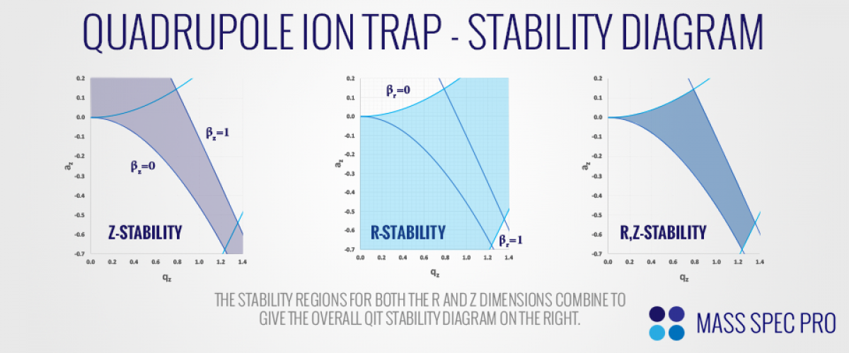
Note that this "stability diagram" is plotted in the $a_z,q_z$ plane, even though it represents stability in both the r and z axes.  This can be slightly confusing.  However, it's helpful if we remember equations 26-29, which show that the values of $a_r$ and $q_r$ are equal to $-2a_z$ and $-2q_z$.  Thus a plot of stability boundaries for the r dimension is inverted and multiplied by two in both directions when plotted on the $a_z$ and $q_z$ axes.  As a result, the QIT's stability diagram is asymmetic about $a_z=0$ axis.  This is in contrast to both the quadrupole mass filter (QMF) and linear ion trap (LIT), which both have stability diagrams that are symmetric about said axis.

Now we can consider the position of ions inside the stability diagram under different experimental conditions, namely different values of DC (U) and RF (V) voltages.  First, consider the situation in which no DC is applied (U=0) and some RF apmlitude, V.  According to equation 26, all ions will posses $a_z$ values of zero, regardless of their mass.  Furthermore, according to equation 27, all ions will have non-zero $q_z$ values, with the heaviest ions having the lowest values and lightest ions having the highest values.  As such, the ions arrange themselves along the $a_z=0$ line of the stability diagram, with the heaviest ions to the left (near $q_z=0$), and lighter ions offset to the right due to their different m values.  If the RF amplitude is increased, the q-values of the ions will scale proportionally, moving them further to the right of the stability diagram.  Then if a negative DC voltage is applied, the ions will move above the $a_z=0$ axis (assuming they're positively charged).  According to equation 26, the degree to which they move is inversely proportional to their mass, with the heaviest ions remaining closer to the axis and lighter ions deviating further up the stability diagram:

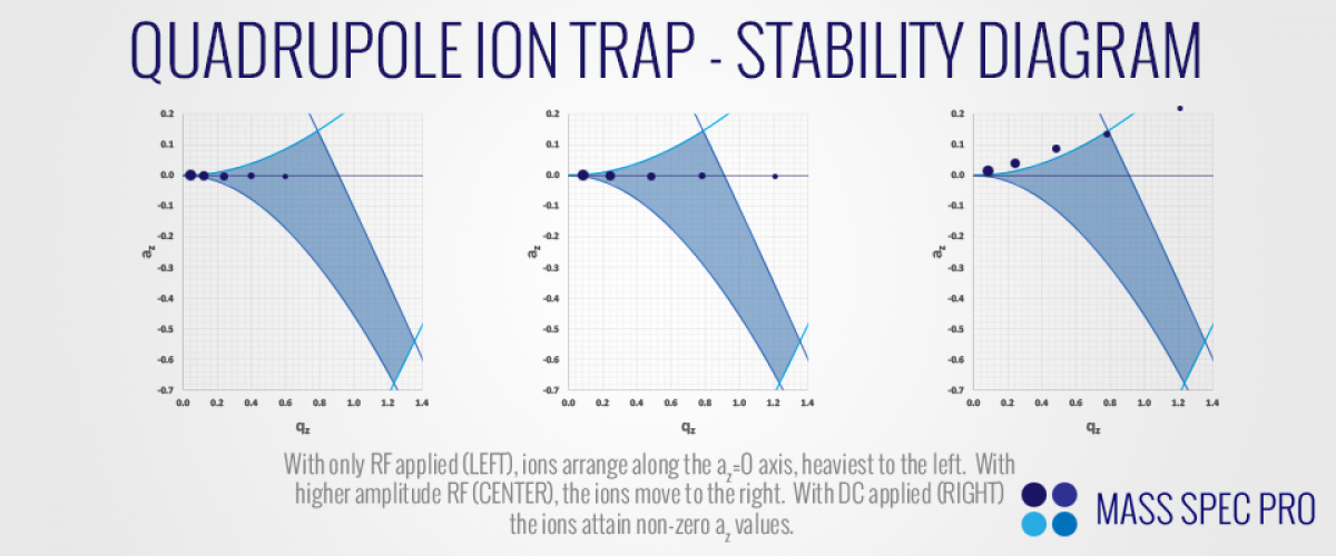
In the right graph of the figure above, note how one of the masses is positioned just under the "apex" of the stability region, while all other masses are outside of the region.  This is actually one of the ways in which the QIT was used as a mass analyzer in the 1960's.  Electrons would enter the center of the trap through holes in either the ring or endcap while RF was applied to the ring.  The electric field inside the trap would accelerate electrons enough to ionize whatever analyte molecules happened to be inside the trap at that time.  If set with an appropriate amplitude, the RF would effectively trap the ions that were generated.  The RF and DC would then be set to put a single m/z value under the apex of the stability diagram.  Following this "isolation" step, the ions that remained stable would be pushed out of the trap with a DC pulse.  The ions would "eject" through a hole in the endcap and strike an electron multiplier detector.  A full mass spectrum could be generated by slightly changing the isolation conditions each time the scan was run.  The number of ions striking the detector in each run of the scan would correspond to the relative abundance of the specific m/z range that had been isolated during that run.  While this methodology was certainly capable of generating mass spectra, it was quite slow and inefficient.  Each time the trap was filled with ions, only a small fraction of the m/z range would be detected.  As such, the QIT was not widely adopted as a mass analyzer.  Despite the QIT's shortcomings at this point in history, the ability to eject ions from the trap and detect them via an electron multiplier paved the way for some remarkable developments in subsequent years.

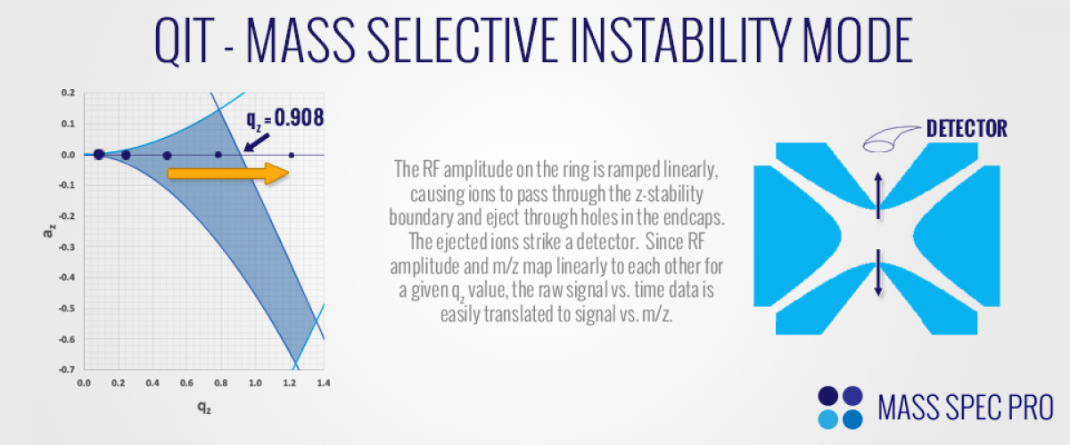
In the early 1908's, a team of scientists and engineers led by George Stafford at Finnigan developed a groundbreaking method of operating the QIT.  The method, described in US Patent #4540884, has since been coined "mass selective instability mode".  As with previous modes of operation, the trap is first filled with ions while RF is applied to the ring.  A range of m/z values will have stable trajectories, based on the various experimental conditions (e.g. RF frequency, amplitude, ion m/z, etc.).  However, instead of isolating a single m/z value under the apex of the stability diagram, the ions are instead pushed to the right of the stability diagram by a linear ramp of the RF amplitude.  This causes ions to cross over the stability boundary at $q_z = 0.908$ in order of increasing m/z.  Since the ions are crossing over the z-stability boundary, they only become unstable in the z-direction.  As such, they can eject through small holes in the endcaps of the trap:

 

ION MOTION

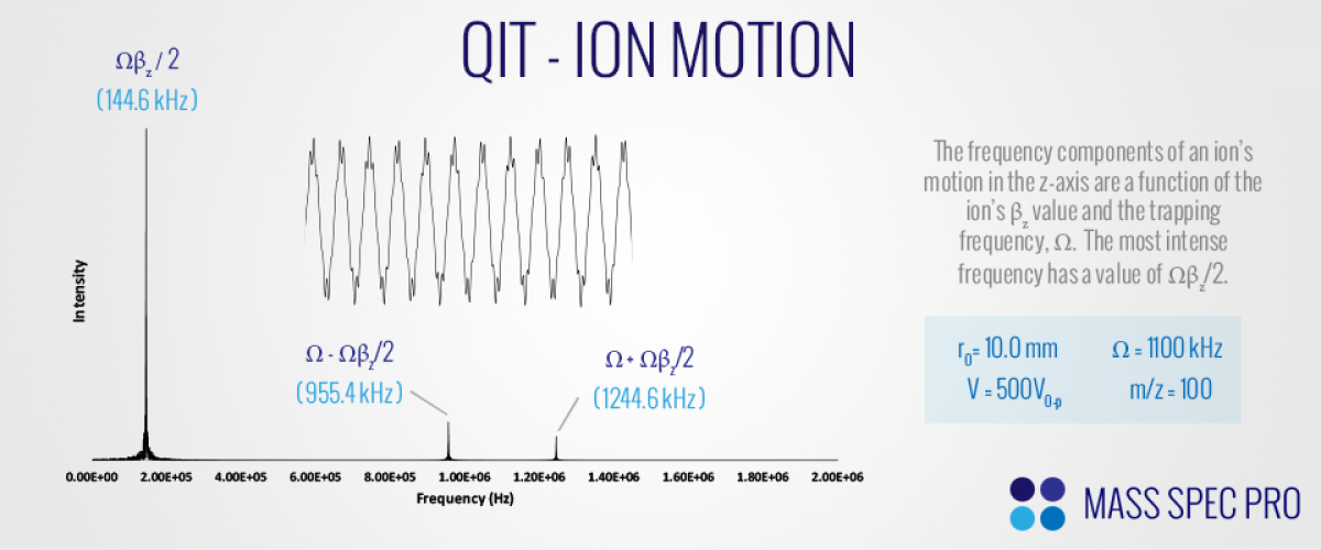
The motion of ions along each axis of a pure quadrupole field are completely independent/decoupled.  Whatever happens to the ion's motion in the z-dimension has no effect on its motion in the r-direction and vice versa.   Ion motion along each axis is rather complex, comprising numerous sinusoidal components in both dimensions.  The frequencies of these components are termed "secular" frequencies, and they are related to the value of $\beta_u$ by:

$$\begin{equation}\omega_{u,n} = \left(n+\frac{1}{2}\beta_u\right)\Omega~~~~~~~~~~0\leq n < \infty \end{equation}$$

$$\begin{equation}\omega_{u,n} = -\left(n+\frac{1}{2}\beta_u\right)\Omega~~~~~~~~~~-\infty < n < 0\end{equation}$$

Since the integer 'n' can range from zero to $\pm \infty$ there are a large number of secular frequencies in any given ion's motion.  However, generally speaking the relative strength of each secular frequency drops very quickly from $n=0$ to $n=\pm 1$, $n=\pm 2$, etc.   Since the "fundamental" (n=0) frequency is the strongest component of a given ion's motion, the term "secular frequency" is typically used to describe this frequency alone.  Since the dominant frequency of ion motion is at a lower frequency than the corresponding higher order components, an ion's motion comprises a low amplitude ripple on top of a more slowly varying sine wave:

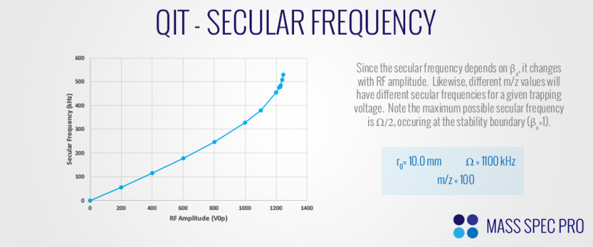
Since the secular frequency in the z-axis is a function of $\beta_z$, ions with different m/z values will possess different secular frequencies for a given RF amplitude. Likewise, as the RF amplitude changes, the secular frequencies of all ions in the trap change accordingly.  It should also be noted that the maximum possible secular frequency that an ion will ever obtain is $\Omega/2$, occuring at the stability boundary:

It's also worth noting that in a pure quadrupole field, the frequencies of ion motion are independent of the ion's position.  For example, an ion's secular frequency in the z-dimension will be the exact same whether the ion is oscillating close to the center of the trap with a small amplitude or deviating far from the center of the trap with a large amplitude.

PSEUDOPOTENTIAL MODEL

Since the main component of ion motion in the QIT is a sine wave, it was recognized in the late 1950's and early 1960's that ions could be approximated as oscillating in a harmonic "pseudopotential well".  Even though the electric field of the QIT is oscillating rapidly with time, its time-averaged effect is essentially a pseudopotential with a restoring force pushing ions toward the center of the trap.  The depth of this pseudopotential well is effectively a measure of how strongly an ion is confined within the trap.  Well depth in the z and r dimensions is given by:

$$\begin{equation}\overline{D_z} = \frac{Vq_z}{8}\end{equation}$$

$$\begin{equation}\overline{D_r} = \frac{Vq_r}{8}\end{equation}$$

From the relationship between $q_r$ and $q_z$ it can be deduced that:

$$\begin{equation}\overline{D_z} = 2\overline{D_r}\end{equation}$$

In other words, ions are confined in a deeper pseudopotential along the z-axis than they are along the r-axis.  Several things should be noted about potential well depths:

• For a given RF amplitude, ions of high m/z will be sitting in shallower potential wells than their lighter counterparts due to their lower q values.
• For an ion of a given m/z, the potential well depth can be increased by raising the RF amplitude.  The deeper well pushes the ions closer to the center of the trap.
• If the RF amplitude is sufficiently low that an ion resides in a very shallow potential well, it could strike the electrodes and be neutralized.  Ions are more easily lost in the radial direction due to the 2x shallower potential well along said axis.
• If a higher RF frequency is used, and the amplitude is scaled accordingly (to keep an ion at the same q value), ions will reside in deeper potential wells.  In other words, higher RF frequencies can translate to stronger trapping of ions.

 

RESONANCE EJECTION/Excitation

Once an ion is confined within the trap by the main RF voltage applied to the ring electrode, the ion's motion can be excited by applying additional waveforms to the trap electrodes.  The ion can pick up energy from the additional fields, causing it to move further away from the center of the trap.  If considering the pseudopotential model, you can think of the ion as being pulled/pushed further up the sides of the potential well.  If the ion's motion is excited sufficiently, the ion can either be ejected or strike an electrode.  How is this excitation accomplished?

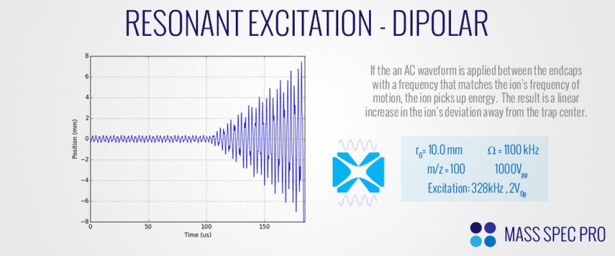
Perhaps the most common methodology is called "dipolar" excitation, in which a low amplitude AC field is applied between the endcaps (with a frequency at or below Ω/2).   Specifically, a low amplitude sine wave is applied to one end cap, while an equal-and-opposite (180 degrees out of phase) sine wave is applied to the other endcap.  If the frequency of these waveforms closely matches the secular frequency of a given m/z, the ion will begin to "resonate" with the additional field, moving further and further from the center of the trap with a linear increase in amplitude with time.

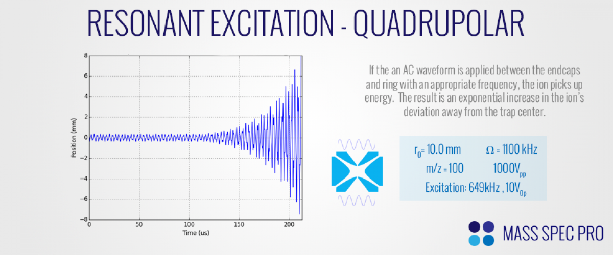
An alternative method of exciting ion trajectories is to apply AC waveforms of the same phase to both endcaps.  This is called "quadrupolar excitation", and it results in an exponential increase in the amplitude of ion motion if an appropriate frequency is used:

The ability to excite an ion's motion and move it away from the center of the trap is one of the most powerful aspects of ion trap operation in mass spectrometry.  It is used in several common modes of operation:

• Resonance Ejection: All commercial ion traps use some variant of "resonance ejection", in which they utilize AC waveforms to eject ions from the trap during the mass analysis step.  Most commonly, bipolar excitation is performed during a linear ramp of the main trapping voltage.  As ions move left to right across the stability diagram, their secular frequencies continually increase.  Eventually their secular frequency approaches the biploar AC's frequency, and the ions begin to resonate and move further from the trap center.  Eventyally the ions have picked up enough energy to eject form the trap altogether.  If done appropriately, resonance ejection can enhance the instrument's mass resolution (in comparison to normal "boundary ejection").
• Broadband Isolation: When performing MS/MS analysis with an ion trap, it is imperative to first isolate the m/z of interest.   All other m/z values can be ejected from the trap by performing resonance excitation with a range of AC frequencies.  If done appropriately (viz. with the correct frequencies omitted), a relatively narrow m/z range can remain in the trap while all others are ejected.
• Fragmentation: As ions move away from the center of the trap, they pick up kinetic energy.  In the event that they subsequently collide with a neutral, there is an elevated amount of energy which can be converted into internal energy.  If enough of these collisions occur, the ion can attain sufficient internal energy to actually break bonds, resulting in fragmentation.  Such fragmentation can be achieved with resonance excitation by applying just enough amplitude to stretch the ion away from the center of the trap without actually ejecting it.  This is critical for MS/MS, which requires both isolation and fragmentation.

 

ION CREATION/INJECTION

Ion traps have to be "filled" with ions prior to peforming mass analysis.  This filling can be accomplished in one of two ways: creating ions directly within the trap or injecting ions into the trap.  These are commonly referred to as "internal ionization" and "external ionization", respectively.  Internal ionization is most often accomplished by leaking analyte neutrals into the ion trap volume and then firing a beam of electrons into the trapping volume (through holes in the endcaps) while RF is applied.  The fate of the electrons as they approach the trap depends on the phase angle of the RF waveform.  During the negative swing of the RF the electrons are repelled and possibly may not even enter the trap.  However, during the positive swing of the RF many electrons will be accelerated into the trapping volume.  If the electrons pick up sufficient kinetic energy, then their collisions with analyte neutrals will cause ionization.  Since the newly made analyte ions are generated inside the trap, the RF field is able to confine the ions, focusing them to the center of the trap where they can be further manipulated/analyzed.  It should be noted that internal ionization is only really applicable to volatile analytes.  For lower volatility analytes, external ionization must be utilized.  A beam of ions is generated outside of the trap through another mechanism (e.g. electrospray, chemical ionization, etc.) and is then injected into the trap (again through holes in the endcaps).  It should be noted that in theory it is impossible to trap externally generated ions without collisions.  As such, there must be some number of neutral molecules (often helium) inside the trap to aid the trapping process.  Much like the electrons of internal ionization, the ions of external ionization will experience different forces depending on the phase angle of the RF as they approach; there are only relatively narrow phase angles within an RF cycle that are amenable to trapping.  The net result is a relatively low trapping efficiency for external ionization.

Automatic Gain Control (AGC)

For both internal and external ionization, the duration of "filling" can be adjusted as desired.  If an insufficient number of ions is trapped, the fill time can be lengthened on the next scan to build up a larger population (e.g. to achieve higher SNR).  Likewise, if too many ions are trapped, the fill time can be dynamically shortened on the next scan to mitigate the side effects (e.g. space charge repulsion between ions).  This is yet another unique feature of ion traps.  When an instrument is in the middle of a large spike in signal, it can throttle fill time down, providing improved dynamic range on the high end.  Then as signal dies down, the instrument can throttle fill time back up, providing ultimate sensitivity and dynamic range on the low end.  Essentially, AGC provides a mechanism that can balance both maximum sensitivity and dynamic range on the fly.  This concept was pioneered by Finnigan Corporation in the late 1980's, and is often referred to as AGC (Automatic Gain Control).  The original US patent (5107109) can be found here.  Similar methodologies have been implemented by other vendors for their ion trap instruments as well.

 

Higher Order Fields

The previous discussion has assumed that the field inside the ion trap is 100% quadrupolar.  However, it is physically impossible to generate such a field.  There are several causes of non-quadrupolar field components within ion traps:

• Electrodes do not extend to infinity
• Holes in endcaps for ion entrance/exit
• Imperfect machining of electrodes
• Imperfect alignment of electrodes

If the fields within the trap retain cylindrical symmetry, then we can account for the non-quadrupolar components by realizing that the actual field can be modeled as a sum of various "multipole" fields.  In other words, the field is a sum of quadrupole, hexapole, octopole, decapole, etc. components:

$$\begin{equation}\Phi(r,z) = \Phi_0\sum_{n=0}^{\infty}A_n\phi_n(r,z)\end{equation}$$

The value of "n" is the "order" of each multipole; n=2 is the quadrupole, n=3 is the hexapole, etc.  The coefficient $A_n$ is a weighting factor for each multipole; the smaller the value, the less that multipole contributes to the overall field inside the trap.  The value of $\phi_n(r,z)$ is the specific electric field distribution associated with each multipole.  In order to determine the mathematical form of these higher order fields we start with the solutions to the Laplace equation in spherical coordinates:

$$\begin{equation}\Phi(\rho,\theta\,\phi) = \Phi_0\sum_{n=0}^{\infty}A_n \frac{\rho^2}{r_0^n}P_n(\cos\theta)\end{equation}$$

In the above equation, $P_n$ is the "Legendre polynomial" of order n, and both $\theta$ and $\rho$ are the polar coordinates.  Note that the potential is assumed to not vary with the coordinate $\phi$ due to its rotational symmetry.  At this point the following basic transforms are useful:

$$\rho^2 = r^2 + z^2$$

$$\cos\theta = \frac{z}{\rho}$$

The "Legendre polynomial" equations of the various orders can be found here.  The equations for n=0 through n=6 have the form:

$$P_0(a) = 1$$

$$P_1(a) = a$$

$$P_2(a) = \tfrac{1}{2}\left(3a^2-1\right)$$

$$P_3(a) = \tfrac{1}{2}\left(5a^3-3a\right)$$

$$P_4(a) = \tfrac{1}{8}\left(35a^4-30a^2+3\right)$$

$$P_5(a) = \tfrac{1}{8}\left(63a^5-70a^3+15a\right)$$

$$P_6(a) = \tfrac{1}{16}\left(231a^6-315a^4+105a^2-5\right)$$

Using all of the above information, the following equations can be derived for the various multipole components:

$$\begin{equation}\phi_0(r,z) = 1\end{equation}$$

$$\begin{equation}\phi_1(r,z) = \frac{z}{r_0}\end{equation}$$

$$\begin{equation}\phi_2(r,z) = \frac{2z^2-r^2}{2r_0^2}\end{equation}$$

$$\begin{equation}\phi_3(r,z) = \frac{2z^3-3zr^2}{2r_0^3}\end{equation}$$

$$\begin{equation}\phi_4(r,z) = \frac{8z^4-24z^2r^2+3r^4}{8r_0^4}\end{equation}$$

$$\begin{equation}\phi_5(r,z) = \frac{8z^5-40z^3r^2+15zr^4}{8r_0^5}\end{equation}$$

$$\begin{equation}\phi_6(r,z) = \frac{16z^6-120z^4r^2+90r^4z^2-5r^6}{16r_0^6}\end{equation}$$

The multipoles "above" quadrupolar are often referred to as "higher order fields".  Any real-world ion trap has a predominantly quadrupolar field with small amounts of higher order multipoles overlayed on top of it.  These higher order components can have very significant effects on ion motion:

• Motion along the axes are coupled: The separation of r and z motion from pure quadrupoles is not strictly true anymore.  Kinetic energy can transfer back and forth between the two dimensions in complex ways.
• Motional frequencies depend on ion position: As ions move away from the center of the trap, their secular frequencies can increase or decrease depending on the nautre of the higher order fields.  This can be advantageous in certain situations.  For example, if secular frequency increases with ion amplitude, then it can actually assist resonance ejection.  As the RF amplitude is ramped, the ion's secular frequency increases until it eventually approaches the resonance ejection frequency.  As it begins to resonate, the ion's motional amplitude will increase.  If the higher order fields then cause the secular frequency to increase, then the ion will move even closer to the resonance ejection frequency, causing it to eject even faster.
• Certain a,q combinations result in "non-linear resonances": Due to a complex interplay between the quadrupole and higher order fields, there are certain conditions that can cause ions to naturally pickup energy from the electric field.  This can cause the ion's motional amplitue to increase significantly.  The increased amplitude can be used as an advantage.  For example, by performing resonance ejection at a non-linear resonance point, both the resonance ejection field and the naturally occurring non-linear resonance work in concert to eject ions faster than they would with resonance ejection alone.