NOTE: This is a working document that is regularly being edited and added to.
In the late 1950's and early 1960's, Wolfgang Paul and collaborators were developing novel methodolgies for storing and manipulating ions through the use of alternating radio frequency electric fields. Their methodologies utilized quadrupolar fields, which by definition have potentials that scale with the square of x,y and z in a cartesian coordinate system:
$$\phi(x,y,z) = A(λx^2 + σy^2 + γz^2) + C$$
Because of the Laplace equation/condition, the gradient of the potential must equal zero (at least in the absence of any charges):
$$\nabla\phi(x,y,z) = 2A(λx + σy + γz) = 0$$
$$λx + σy + γz = 0$$
This equation can be satisfied in an infinite number of ways, with various values of the coefficients λ, σ and γ. One of the most well-known solutions utilizes the combination λ=1, σ=-1 and γ=0 to give a potential of:
$$\phi(x,y) = A(x^2 - y^2) + C$$
This is the basis of the potential inside the now famous quadrupole mass filter (QMF). This potential is best generated via four rods of hyperbolic cross section arranged around a center axis. The "x electrodes" have the form:
$$x^2 - y^2 = r_0^2$$
and the "y electrodes" have the form:
$$y^2 - x^2 = r_0^2$$
In order to determine what the coefficients 'A' and 'C' are, we must consider the boundary conditions of the electrode surfaces themselves. For example, assume that there is a potential $\phi_0$ applied between the two rod sets, with $\frac{\phi_0}{2}$ applied to the x-electrodes and an opposite potential $\frac{-\phi_0}{2}$ applied to the y-electrodes. The equal and opposite voltages cancel out in the center of the rods, giving a value of C=0 in the potential:
$$\phi(x,y) = A(x^2 - y^2)$$
The innermost point of the x-electrodes is located at x=r0 and y=0, and has a potential of $\frac{\phi_0}{2}$:
$$\phi(r_0,0) = \frac{\phi_0}{2} = Ax^2 = Ar_0^2$$
This gives a value of A:
$$A = \frac{\phi_0}{2r_0^2}$$
A similar examination of the potential on the y-electrodes gives the same value for A. As such, the general potential in the QMF has the form:
$$\phi(x,y) = \frac{\phi_0(x^2 - y^2)}{2r_0^2}$$
Now that we have determined the form of the potential as a funciton of x and y, we can consider what happens with the potentials that are usually applied to QMFs. These potentials have both a static DC component and a time varying RF component:
$$\phi_0 = 2(U + VcosΩt)$$
Remember that $\phi_0$ is the difference in potential between the rods, which have equal and opposite potentials applied. This means that the DC component (2U) is split, such that one pair of rods has a DC component of +U and the other pair has -U. Likewise, the RF component (2VcosΩt) is split between the rods; this is accomplished by applying sinusoids of equal and opposite amplitude (V and -V) to the rod pairs. With all these considerations applied, one set of rods has the potential +(U + VcosΩt) applied while the other has the potential -(U + VcosΩt) applied.
Ion Motion in a Quadrupolar Field
Let's consider the motion of an ion in the x dimension, specifically with an ion on the x-axis (y=0). The potential along this axis is:
$$\phi(x,0) = \frac{\phi_0 x^2}{2r_0^2}$$
The electric field along the x-axis at this point is the derivate of the potential:
$$E_x = \frac{d\phi}{dx} = \frac{\phi_0 x}{r_0^2}$$
The force acting on the ion along this axis is determined by multiplying the electric field by -e:
$$F_x = -eE_x = \frac{-e\phi_0 x}{r_0^2}$$
The classic equation F=ma can be applied here:
$$F_x = ma = m\frac{d^2x}{dt^2} = \frac{-e\phi_0 x}{r_0^2}$$
Now we can insert the usual form of $\phi_0 = 2(U + VcosΩt)$:
$$m\frac{d^2x}{dt^2} = \frac{-2e(U + VcosΩt) x}{r_0^2}$$
In preparation for what's to come, this equation is slightly rearranged:
$$m\frac{d^2x}{dt^2} = -\left(\frac{2eU}{r_0^2} + \frac{2eVcosΩt}{r_0^2}\right) x$$
$$\frac{d^2x}{dt^2} + \left(\frac{2eU}{mr_0^2} + \frac{2eVcosΩt}{mr_0^2}\right) x = 0$$
Interestingly, this equation of ion motion has the form of the "Mathieu equation", which is:
$$\frac{d^2u}{d\xi^2} + \left(a_u -2q_ucos2 \xi \right)u=0$$
In order to make the equation of ion motion fit the Mathieu equation format exactly, we make the following substitutions:
$$u=x$$
$$\xi = \frac{\Omega t}{2}$$
$$a_x = \frac{8eU}{mr_0^2 \Omega^2}$$
$$q_x = \frac{-4eV}{mr_0^2 \Omega^2}$$
Similar considerations can be made for ion motion along the y-axis of the QMF, again providing an equation of motion that takes the form of a Mathieu equation with the values:
$$a_y = \frac{-8eU}{mr_0^2 \Omega^2}$$
$$q_y = \frac{4eV}{mr_0^2 \Omega^2}$$
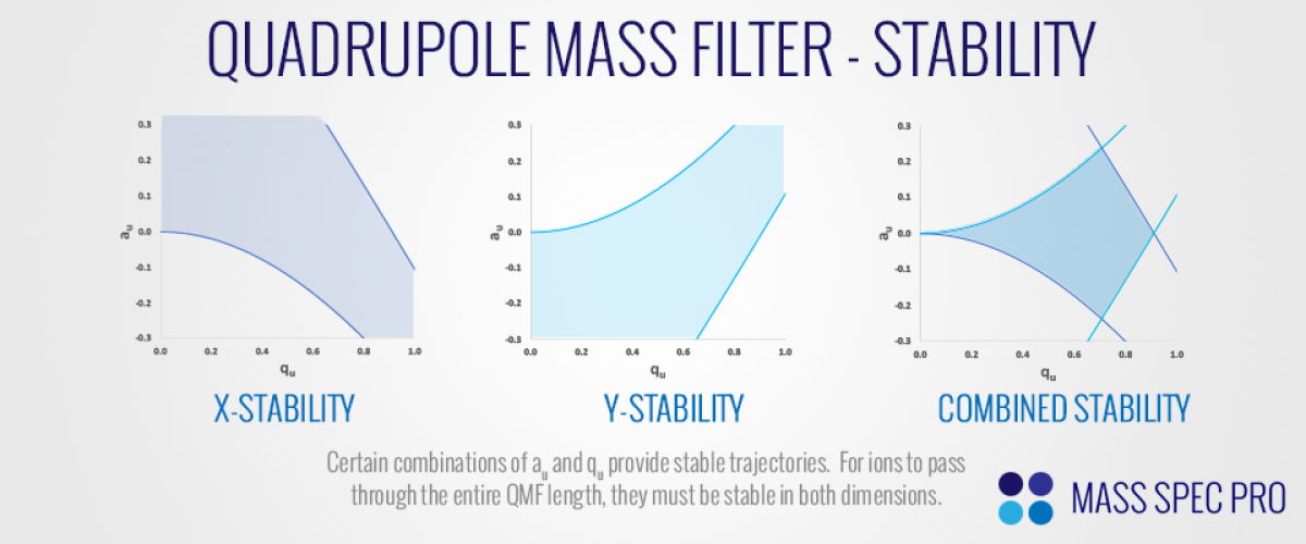
Since the equation of ion motion along the x-axis of the QMF fits the form of the Mathieu equation, we can utilize known characteristics of said equation to think about ion trajectories inside the mass filter. The solutions to the Mathieu equation can be characterized as either "bounded" or "unbounded", based on how their amplitudes evolve over time. There are only certain combinations of $a_u$ and $q_u$ that provide bounded/stable solutions. As such, there are only certain values of $a_x$, $q_x$, $a_y$, and $q_y$ that provide stable ion trajectories As ions fly down the long z-axis of a QMF, they must have stable trajectories in both the x and y dimensions so that they don't strike the metal rods and neutralize. When thinking about these aspects of ion trajectories, it is common to use a "stability diagram" that helps visualize the values of a and q that allow ions to be stable in both the x and y dimensions:
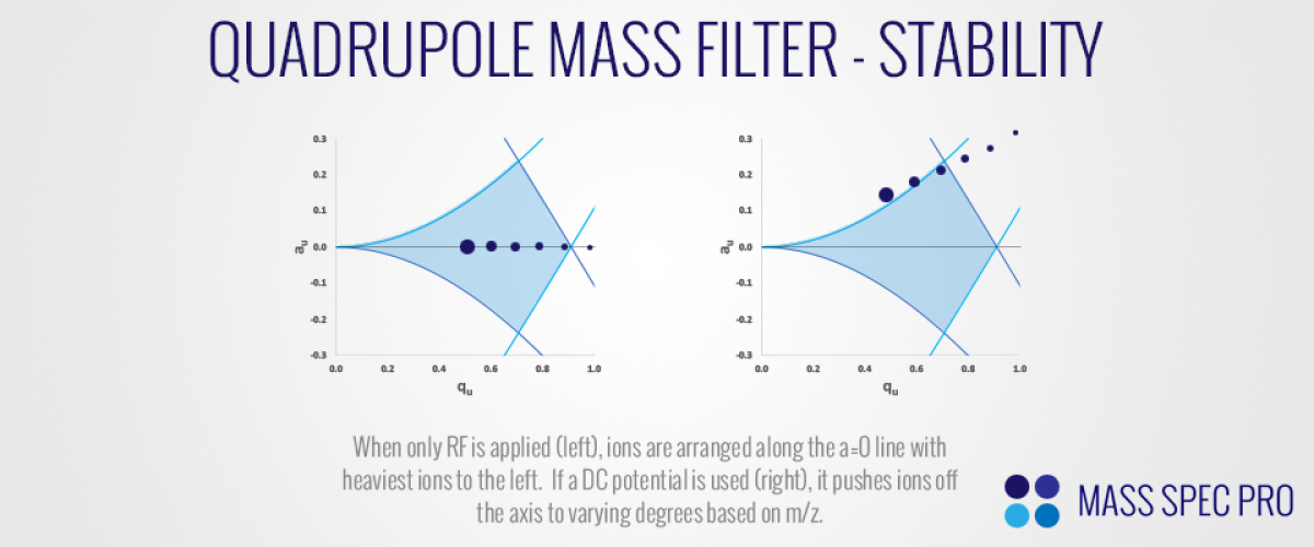
Now let us consider how ions of different m/z values are arranged within the stability diagram. We begin by considering the case when only RF is applied, with no DC difference between the rods (U=0). Since there is no DC applied, the "a-values" for ions of any m/z are zero $(a_x=a_y=0)$. However, since the "q-values" of the ions are m/z-dependent, ions of different masses spread out along the a=0 axis, with heaviest ions to the left and lightest ions to the right. The amplitude of the RF voltage dictates how far to the right ions are pushed. Higher RF amplitudes increase the q-values of all ions, pushing ions to the right in the stability diagram. If the RF amplitude is increased enough, it eventually pushes ions out of the region of stability (with the lightest ions reaching instability first). Once a DC difference is applied between the rods, ions obtain a-values which are inversely proportional to their m/z. Depending on how far ions are pushed up the a-axis, they can exit the region of stability:
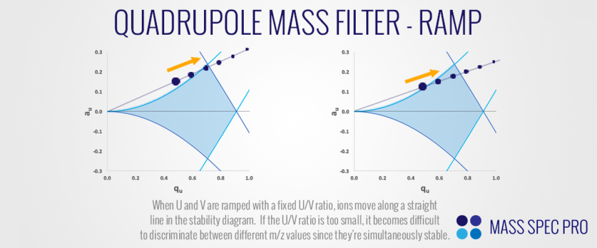
In the right of the preceeding figure, it is apparent that if appropriate RF and DC voltages are applied to the QMF's rods, then only a small subset of m/z values will reside within the region of stability. Notice how only one of our representative ions falls within the region of stability, falling just inside its apex. Meanwhile, ions of both lower and higher m/z values are outside of the stability region. If such conditions were used on a QMF filter, the heavier and lighter ions would quickly become unstable and strike the rods, while the ions just insde the apex would be successfully transmitted through the filter thanks to their stable trajectories. This is the essence of how QMFs perform mass analysis. A beam of ions with various m/z values continuously enters the filter while the RF and DC voltages are ramped together. If the ratio of U and V is held constant, then ions are effectively pushed along a single line within the stability diagram, continually shifting up and to the right. If the U/V ratio is set properly, then ions will pass just under the apex of the stability digram, ensuring good discrimination between nearby m/z values. If the U/V ratio is set too high, then ions simply never pass through the stability region and therefore aren't detected. Lastly, if the U/V ratio is set too low, then ions do not approach the apex of the stability boundary, meaning that a relatively wiude range of m/z values are stable at any given time, causing mass resolution to degrade.
Coming Soon
- Mass Resolution
- Pre/Post Filters
- RF-only QMF
- Triple Quadrupoles